24.1 Random walk redux

In our random walk derivation in Section 23 we focused on the position of a particle on the random walk, based upon prescribed rules. In this scenario we instead are going to consider the probability that a particle is at position \(x\) in time \(t\). We will denote this probability as \(p(x,t)\). In other words, rather than focusing on where the particle is, we focus on the chance that the particle is at a given spot.

A way to conceptualize this is at any given position \(x\), a particle can arrive there from either the left or the right, illustrated in Figure 24.1.

Figure 24.1: Schematic diagram for one-dimensional random walk.

Notice how the the particle in Figure 24.1 could only move in unit increments. To generalize this setup a little more where to increments \(\Delta x\), the equation that defines the probability \(p\) of being at position \(x\) at any time \(t\) is the following:

\[\begin{equation} p(x,t+\Delta t) = \frac{1}{2} p(x-\Delta x,t) + \frac{1}{2} p(x+\Delta x,t) \tag{24.1} \end{equation}\]

The next step to analyze this expression is apply Taylor approximations on each side of Equation (24.1). First let’s do a locally linear approximation for \(p(x,t+\Delta t)\):

\[\begin{equation} p(x,t+\Delta t) \approx p(x,t) + \Delta t \cdot p_{t}, \end{equation}\]

where we have dropped the shorthand \(p_{t}(x,t)\) as \(p_{t}\). On the right hand side of Equation (24.1) we will compute the 2nd degree (quadratic) Taylor polynomial:

\[\begin{align*} \frac{1}{2} p(x-\Delta x,t) & \approx \frac{1}{2} p(x,t) - \frac{1}{2} \Delta x \cdot p_{x} + \frac{1}{4} (\Delta x)^{2}\cdot p_{xx} \\ \frac{1}{2} p(x+\Delta x,t) & \approx \frac{1}{2} p(x,t) + \frac{1}{2} \Delta x \cdot p_{x} + \frac{1}{4} (\Delta x)^{2} \cdot p_{xx} \end{align*}\]

With these approximations we can re-write Equation (24.1) as Equation (24.2):

\[\begin{equation} \Delta t \cdot p_{t} = \frac{1}{2} (\Delta x)^{2} p_{xx} \rightarrow p_{t} = \frac{1}{2} \frac{(\Delta x)^{2}}{\Delta t} \cdot p_{xx} \tag{24.2} \end{equation}\]

Equation (24.2) is called a partial differential equation - what this means is that it is a differential equation with derivatives that depend on two variables (\(x\) and \(t\) (two derivatives). Equation (24.2) is called the diffusion equation. Cool!

We can also simplify Equation (24.2) even more by defining \(\displaystyle D = \frac{1}{2} \frac{(\Delta x)^{2}}{\Delta t}\), so we have \(p_{t}=D \cdot p_{xx}\). Other derivations of the diffusion equation let \(\Delta t \rightarrow 0\) and \(\Delta x \rightarrow 0\) in the limit, but because of Equation (24.2) is connected to a random walk we will not make that limiting argument.

Determining an exact solution to the diffusion equation requires more study in techniques of partial differential equations, so we will leave that for another time. However, the solution to Equation (24.2) is given by Equation (24.3): \[\begin{equation} p(x,t) = \frac{1}{\sqrt{4 \pi Dt} } e^{-x^{2}/(4 D t)} \tag{24.3} \end{equation}\]

Figure 24.2 shows plots for \(p(x,t)\) when \(D=0.5\) (we will call these plots profiles) for different values of \(t\): What Equation (24.3) represents is the probability that the particle is at the position \(x\) at time \(t\). In the exercises for this section you will examine more properties of the diffusion equation.

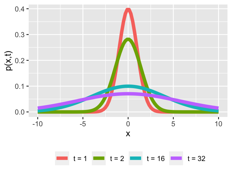
Figure 24.2: Profiles of \(p(x,t)\) (solution to the diffusion equation) for different values of \(t\) with \(D = 0.5\).

As you can see that as time increases the graph of \(p(x,t)\) gets flatter - or more uniform. What this tells you is that the longer \(t\) increases it is less likely to find the particle at the origin.

24.1.1 Verifying the solution to the diffusion equation

Verifying Equation (24.3) is the solution to Equation (24.2) is a good review of your multivariable calculus skills! As a first step to verifying this solution, let’s take the partial derivative with respect to \(x\) and \(t\).

First we will compute \(\displaystyle \frac{\partial p}{\partial x}\) (also represented as \(p_{x}\)): \[\begin{align*} p_{x} &= \frac{\partial }{\partial x} \left( \frac{1}{\sqrt{4 \pi Dt} } e^{-x^{2}/(4 D t)} \right) \\ &= \frac{1}{\sqrt{4 \pi Dt} } e^{-x^{2}/(4 D t)} \cdot \frac{-2x}{4Dt} \end{align*}\]

Notice something interesting here: \(\displaystyle p_{x} = p(x,t) \cdot \left( \frac{-x}{2Dt} \right)\).

To compute the second derivative, we have the following expressions by applying the product rule:

\[\begin{align*} p_{xx} &= p_{x} \cdot \left( \frac{-x}{2Dt} \right) - p(x,t) \cdot \left( \frac{1}{2Dt} \right) \\ &= p(x,t) \cdot \left( \frac{-x}{2Dt} \right) \cdot \left( \frac{-x}{2Dt} \right)- p(x,t) \cdot \left( \frac{1}{2Dt} \right) \\ &= p(x,t) \left( \left( \frac{-x}{2Dt} \right)^{2} - \left( \frac{1}{2Dt} \right) \right) \\ &= p(x,t) \left( \frac{x^{2}-2Dt}{(2Dt)^{2}}\right). \end{align*}\]

So far so good. Now computing \(p_{t}\) gets a little tricky because this derivative involves both the product rule with the chain rule in two places (the variable \(t\) appears twice in the formula for \(p(x,t)\)). To aid in computing the derivative we identify two functions \(\displaystyle f(t) = \frac{1}{\sqrt{4 \pi Dt} } = (4 \pi D t)^{-1/2}\) and \(\displaystyle g(t)= \frac{-x^{2}}{4Dt} = -x^{2} \cdot (4Dt)^{-1}\). This changes \(p(x,t)\) into \(p(x,t) = f(t) \cdot e^{g(t)}\). In this way \(p_{t} = f'(t) \cdot e^{g(t)} + f(t) \cdot e^{g(t)} \cdot g'(t)\). Now we can focus on computing the individual derivatives \(f'(t)\) and \(g'(t)\) (after simplification - be sure to verify these on your own!):

\[\begin{align*} f'(t) &= -\frac{1}{2} (4 \pi D t)^{-3/2} \cdot 4 \pi D = -2\pi D \; (4 \pi D t)^{-3/2} \\ g'(t) &= x^{2}\; (4Dt)^{-2} 4D = \frac{x^{2}}{4Dt^{2}} \end{align*}\]

Assembling these results together, we have the following:

\[\begin{align*} p_{t} &= f'(t) \cdot e^{g(t)} + f(t) \cdot e^{g(t)} \cdot g'(t) \\ &= -2\pi D \; (4 \pi D t)^{-3/2} \cdot e^{-x^{2}/(4 D t)} + \frac{1}{\sqrt{4 \pi Dt} } \cdot e^{-x^{2}/(4 D t)} \cdot \frac{x^{2}}{4Dt^{2}} \\ &= \frac{1}{\sqrt{4 \pi Dt} } \cdot e^{-x^{2}/(4 D t)} \left( -2 \pi D \; (4 \pi D t)^{-1} + \frac{x^{2}}{4Dt^{2}} \right) \\ &= \frac{1}{\sqrt{4 \pi Dt} } \cdot e^{-x^{2}/(4 D t)} \left( -\frac{1}{2t} + \frac{x^{2}}{4Dt^{2}} \right) \\ &= p(x,t) \left( -\frac{1}{2t} + \frac{x^{2}}{4Dt^{2}} \right) \end{align*}\]

Wow. Verifying Equation (24.3) is a solution to the diffusion equation is getting complicated, but also notice that through algebraic simplification, \(\displaystyle p_{t} = p(x,t) \left(\frac{x^{2}-2Dt}{4Dt^{2}} \right)\). If we compare \(p_{t}\) to \(D p_{xx}\), they are equal!

The connections between diffusion and probability are so strong. Equation (24.3) is related to the formula for a normal probability density function (you might want to refer back to Section 9)! In this case, the standard deviation in Equation (24.3) dependent on time (Exercise 24.2). Even though we approached the random walk differently here compared to Section 23, we also saw that the variance grew proportional to the time spent, so there is some consistency.