6.3 Generating a phase plane in R | Exploring Modeling with Data and Differential Equations Using R

6.3 Generating a phase plane in `R`

Let’s take what we learned from the case study of the flu model with quarantine to qualitatively analyze a system of differential equations:

We determine nullclines by setting the derivatives equal to zero.
Equilibrium solutions occur where nullclines for the two different equations intersect.
The arrows in the phase plane help us characterize the stability of the equilibrium solution.

To determine the phaseplane diagram demodelr package has some basic functionality to generate a phase plane. Consider the following system of differential equations (Equation (6.3)):

\[\begin{equation} \begin{split} \frac{dx}{dt} &= x-y \\ \frac{dy}{dt} &= -x+y \end{split} \tag{6.3} \end{equation}\]

In order to generate a phaseplane diagram for Equation (6.3) we need to define functions for $x'$ and $y'$, which I will annotate as $dx$ and $dy$ respectively. We are going to collect these equations in one vector called system_eq, using the tilde (~) as a replacement for the equals sign:

system_eq <- c(dx ~ x-y,
               dy ~ x+y)

Then what we do is apply the command phaseplane, which will generate a vector field over a domain:

phaseplane(system_eq,'x','y')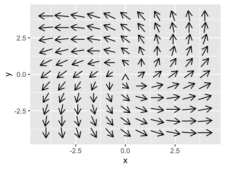

$Phaseplane diagram for Equation \@ref(eq:phase-example)$

Figure 6.5: Phaseplane diagram for Equation (6.3)

# The values in quotes are the labels for the axes and to identify the variables - they are needed!

The command phaseplane has an option called eq_soln that will if there are any equilibrium solutions to be found and report them to the console. For example try running phaseplane(system_eq,'x','y',eq_soln=TRUE) and see what gets output to console. While this option lists equilibrium solutions, you should confirm them with the differential equation through direct solving.

6.3.1 Generating a phase line in R:

From Section 5 we discussed how to construct phaselines by hand. It turns out that the command phaseplane can also plot phase lines. Let’s take a look at an example first and then discuss how that it works.

Example 6.1 A colony of bacteria growing in a nutrient-rich medium deplete the nutrient as they grow. As a result, the nutrient concentration $x(t)$ is steadily decreasing. Determine the phaseline for the following differential equation:

# Define the windows where we make the plots
t_window <- c(0,3)
x_window <- c(0,5)

# Define the differential equation
system_eq <- c(dt ~ 1,
               dx ~ -0.7 * x*(3-x)/(1+x))

phaseplane(system_eq,"t","x",t_window,x_window)

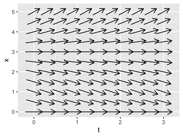
Notice how we have the equation $dt = 1$. What we are doing is re-writing the differential equation with a new variable $s$ (Equation (6.5)):

\[\begin{equation} \begin{split} \frac{dt}{ds} &= 1 \\ \frac{dx}{ds} &= - 0.7 \cdot \frac{x \cdot (3- x)}{1 + x} \end{split} \tag{6.5} \end{equation}\]

The differential equation $\displaystyle \frac{dt}{ds} = 1$ has solution $s=t$, so in essence is the same as Equation (6.4) (perhaps a little more complicated). However re-writing this system was a quick and handy workaround to re-use code.