17.2 The lynx hare revisited
Let’s take a look at another familiar example. Consider the following nonlinear system of equations from the Lynx-Hare model, with \(H\) and \(L\) measured in thousands of animals:
\[\begin{equation} \begin{split} \frac{dH}{dt} &= .3 H - .1 HL \\ \frac{dL}{dt} &=.05HL -.2L \end{split} \tag{17.2} \end{equation}\]
You can show that the steady states for Equation (17.2) are \((H,L)=(0,0)\) and \((4,3)\). The phase plane diagram for this system is the following:
# Define the range we wish to evaluate this vector field
H_window <- c(0,5)
L_window <- c(0,5)

system_eq <- c(dH ~ .3*H - .1*H*L,
               dL ~ .05*H*L -.2*L)

# Reminder: The values in quotes are the labels for the axes
phaseplane(system_eq,'H','L',x_window = H_window, y_window = L_window) 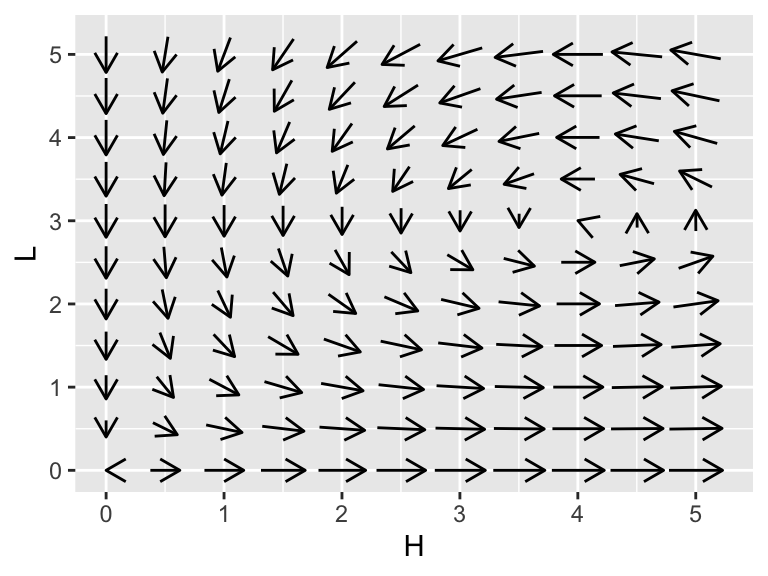
Let’s take a closer look at the phase plane near the first equilibrium solution:
# Define the range we wish to evaluate this vector field
H_window <- c(0,0.5)
L_window <- c(0,0.5)

system_eq <- c(dH ~ .3*H - .1*H*L,
               dL ~ .05*H*L -.2*L)

# Reminder: The values in quotes are the labels for the axes
phaseplane(system_eq,'H','L',x_window = H_window, y_window = L_window) 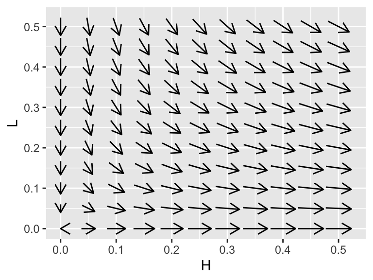
Figure 17.2: A zoomed in view of the lynx-hare system.
While the phaseplane in Figure 17.2 looks like this equilibrium solution is unstable, verifying this with another approach would be useful. To do so, we are going to do a locally linear approximation or tangent plane approximation around \(H=0\), \(L=0\), which we discuss next.